Original title: “Exploring circle STARKs” Written by Vitalik Buterin, Ethereum co-founder compiled by Chris, Techub News
The premise of understanding this article is that you have already understood the basic principles of SNARKs and STARKs.If you are not familiar with this, it is recommended that you read the first few parts of this article to learn the basics.
In recent years, the trend of STARKs protocol design is to shift to using smaller fields.The earliest STARKs production implementations used 256-bit fields, which were modular operations on large numbers (such as 21888…95617), which made these protocols compatible with elliptic curve-based signatures.However, this design is relatively inefficient. Generally speaking, processing and calculating these large numbers has no practical purpose, and it will waste a lot of computing power, such as processing X (representing a certain number) and processing four times X, processing XOnly one-ninth of the calculation time is required.To solve this problem, STARKs began to turn to smaller fields: first Goldilocks, then Mersenne31 and BabyBear.
This shift improves proof speed, such as Starkware’s ability to prove 620,000 Poseidon2 hashes per second on an M3 laptop.This means that as long as we are willing to trust Poseidon2 as a hash function, we can solve the problem in developing efficient ZK-EVM.So how do these technologies work?How do these proofs be established on smaller fields?How do these protocols compare to solutions like Binius?This article will explore these details, focusing specifically on a scheme called Circle STARKs (stwo in Starkware, plonky3 in Polygon, and my own version implemented in Python), which has unique properties that are compatible with the Mersenne31 field.
Common Problems When Using Smaller Math Fields
When creating hash-based proofs (or any type of proof), a very important technique is to indirectly verify the properties of polynomials by proofing the results of the evaluation of polynomials at random points.This approach can greatly simplify the proof process, as evaluation at random points is usually much easier than dealing with the entire polynomial.
For example, suppose a proof system requires you to generate a commit for polynomials, A, must satisfy A^3 (x) + x – A (\omega*x) = x^N (a very common one in the ZK-SNARK protocolproof type).The protocol can ask you to select a random coordinate? and prove that A (r) + r – A (\omega*r) = r^N.Then invert A (r) = c, you prove that Q = \frac {A – c}{X – r} is a polynomial.
If you understand the details of the protocol or the internal mechanisms in advance, you may find ways to bypass or crack these protocols.Specific operations or methods may be mentioned next to achieve this.For example, to satisfy the A (\omega * r) equation, you can set A (r) to 0 and then make A a straight line passing through these two points.
To prevent these attacks, we need to select r after the attacker provides A (Fiat-Shamir is a technology used to enhance protocol security, avoiding attacks by setting certain parameters to a certain hash value.The parameters need to come from a large enough set to ensure that the attacker cannot predict or guess these parameters, thereby improving the security of the system.
In the elliptic curve-based protocol and STARKs in the 2019 period, this problem is simple: all our maths are performed on 256-bit numbers, so we can select r as a random 256-bit number so that we can do itNow.However, in STARKs on smaller fields, we have a problem: there are only about 2 billion possible r values to choose from, so an attacker who wants to forge proofs only needs to try 2 billion times, although the workload is high, but for an attacker who is determined, it can still be done!
There are two solutions to this problem:
-
Perform multiple random checks
-
Extended fields
The simplest and most effective way to perform multiple random checks: instead of checking on one coordinate, it is better to check on four random coordinates repeatedly.This is theoretically feasible, but there are efficiency issues.If you are dealing with a polynomial with a degree smaller than a certain value and operating on a domain of a certain size, an attacker can actually construct a malicious polynomial that looks normal in these positions.Therefore, whether they can successfully break the protocol is a probabilistic question, so the number of rounds of checks needs to be increased to enhance overall security and ensure effective defense against attackers.
This leads to another solution: Extended domain, Extended domain is similar to plural, but it is based on finite domains.We introduce a new value, denoted as α\alphaα, and declare that it satisfies a certain relationship, such as α2=some value\alpha^2 = \text {some value}α2=some value.In this way, we create a new mathematical structure that enables more complex operations on finite domains.In this extended domain, the calculation of multiplication becomes a multiplication using the new value α\alphaα.We can now manipulate value pairs in extended domains, not just single numbers.For example, if we work on fields like Mersenne or BabyBear, such an extension allows us to have more value choices, thus improving security.To further increase the size of the field, we can repeatedly apply the same technique.Since we have used α\alphaα, we need to define a new value, which in Mersenne31 manifests as selecting α\alphaα such that α2=some value\alpha^2 = \text {some value}α2=some value.
Code (you can improve it with Karatsuba)
By extending the domain, we now have enough values to choose to meet our security needs.If you are dealing with a polynomial with a degree smaller than ddd, each round can provide 104-bit security.This means we have sufficient security.If you need to reach a higher security level, such as 128 bits, we can add some additional computing work to the protocol to enhance security.
Extended domains are only used in FRI (Fast Reed-Solomon Interactive) protocol and other scenarios that require random linear combinations.Most mathematical operations are still performed on basic fields, which are usually fields that are modulo ppp or qqq.Meanwhile, almost all hashed data is done on the base field, so each value only has four bytes hashed.Doing so can take advantage of the efficiency of small fields, while using larger fields when security enhancements are required.
Regular FRI
When building SNARK or STARK, the first step is usually arithmetization.This is to translate arbitrary computational problems into an equation where some variables and coefficients are polynomials.Specifically, this equation will usually look like P (X,Y,Z)=0P (X,Y,Z)=0, where P is a polynomial, X,Y, andZ is the given parameter, and the solver needs to provide the values of X and Y.Once such an equation is present, the solution of the equation corresponds to the solution of the underlying computational problem.
To prove that you have a solution, you need to prove that the value you propose is indeed a reasonable polynomial (rather than a fraction, or in some places it looks like a polynomial and in other places it is a different polynomial, etc.),And these polynomials have a certain maximum degree.To do this, we use a step-by-step random linear combination technique:
-
Suppose you have an evaluation value of polynomial A, and you want to prove that its degree is less than 2^{20}
-
Consider polynomial B (x^2) = A (x) + A (-x), C (x^2) = \frac {A (x) – A (-x)}{x}
-
D is a random linear combination of B and C, i.e. D=B+rCD = B + rCD=B+rC, where r is a random coefficient.
Essentially, what happens is B isolates even coefficients A, and? isolates odd coefficients.Given B and C, you can restore the original polynomial A: A (x) = B (x^2) + xC (x^2).If the degree of A is indeed less than 2^{20}, then the degrees of B and C will be the degrees of A and the degrees of A, respectively, minus 1.Because the combination of even and odd terms does not increase the degree.Since D is a random linear combination of B and C, the degree of D should also be the degree of A, which allows you to verify whether the degree of A meets the requirements by the degree of D.
First, FRI simplifies the verification process by simplifying the problem of proving polynomial degree of d to the problem of proving polynomial degree of d/2.This process can be repeated several times, simplifying the problem halfway each time.
The working principle of FRI is to repeat this simplified process.For example, if you start with proof that the polynomial is d, through a series of steps, you will eventually proof that the polynomial is d/2.After each simplification, the degree of the generated polynomial is gradually reduced.If the output of a stage is not the expected polynomial degree, this round of checks will fail.If someone tries to push a polynomial that is not a degree d through this technique, then in the second round of output, the degree will have a certain probability that it will not meet expectations, and in the third round, there will be more likely to be a non-conformity situation.The check will fail.This design can effectively detect and reject inputs that do not meet the requirements.If the dataset is equal to a polynomial with a degree d at most locations, this dataset has the potential to be validated by FRI.However, in order to construct such a data set, an attacker needs to know the actual polynomial, so even a slight flawed proof indicates that the prover is able to generate a “real” proof.
Let’s take a closer look at what’s going on here and the properties needed to make this work.In each step, we reduce the number of polynomials by half, while also reducing the set of points (the set of points we focus on) by half.The former is the key to making the FRI (Fast Reed-Solomon Interactive) protocol work properly.The latter makes the algorithm run extremely fast: since the scale of each round is reduced by half compared to the previous round, the total calculation cost is O (N), not O (N*log (N)).
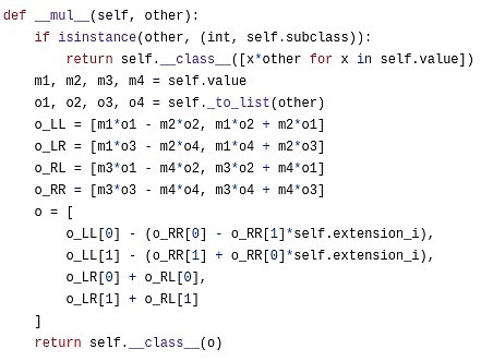
To achieve a gradual reduction in the domain, a two-to-one mapping is used, i.e., each point is mapped to one of the two points.This mapping allows us to reduce the size of our dataset in half.An important advantage of this two-to-one mapping is that it is repeatable.That is, when we apply this mapping, the resulting result set still retains the same properties.Suppose we start with a multiplicative subgroup.This subgroup is a set S where each element x has its multiple 2x in the set as well.If you perform a square operation on set S (i.e. map each element x in the set to x^2), the new set S^2 retains the same attributes.This operation allows us to continue reducing the size of the dataset until we end up with only one value left.Although in theory we can narrow down the dataset to only one value left, in practice, it will usually stop before a smaller set is reached.
You can think of this operation as a process of extending a line (for example, a segment or an arc) on the circumference, causing it to rotate two turns around the circumference.For example, if a point is at a x degree position on the circumference, then after this operation, it moves to a 2x degree position.Each point on the circumference has a corresponding point at 180 to 359 degrees, and these two points will overlap.This means that when you map a point from x to 2x degrees, it coincides with a position at x+180 degrees.This process can be repeated.That is, you can apply this mapping operation multiple times, each time moving points on the circumference to their new position.
To make the mapping technique effective, the size of the original multiplication subgroup needs to have a large power of 2 as a factor.BabyBear is a system with a specific modulus whose modulus is a value such that its maximum multiplication subgroup contains all nonzero values, so the size of the subgroup is 2k−1 (where k is the number of bits of the modulus).This sized subgroup is very suitable for the above technique because it allows the degree of the polynomial to be effectively reduced by repeatedly applying mapping operations.In BabyBear, you can select a subgroup of size 2^k (or directly use the entire set), then apply the FRI method to gradually reduce the degree of the polynomial to 15, and check the degree of the polynomial at the end.This method utilizes the properties of the modulus and the size of multiplication subgroups, making the calculation process very efficient.Mersenne31 is another system with a modulus of some value, such that the size of the multiplication subgroup is 2^31 – 1.In this case, the multiplication subgroup has only one power of 2 as a factor, which makes it only divide by 2 once.The subsequent processing no longer applies to the above techniques, that is, it is impossible to use FFT to perform effective polynomial degree reduction like BabyBear.
The Mersenne31 domain is ideal for arithmetic operations in existing 32-bit CPU/GPU operations.Because of its modulus characteristics (for example, 2^{31} – 1), many operations can be accomplished using efficient bit operations: if the result of adding two numbers exceeds the modulus, you can shift the result from the modulus.Operation to reduce to the appropriate range.Displacement operation is a very efficient operation.In multiplication operations, specific CPU instructions (usually called high-bit displacement instructions) can be used to process the results.These instructions can efficiently calculate the high-bit portion of the multiplication, thereby improving the efficiency of the operation.In the Mersenne31 domain, due to the above characteristics, arithmetic operations are about 1.3 times faster than in the BabyBear domain.Mersenne31 provides higher computing efficiency.If FRI can be implemented in the Mersenne31 domain, this will significantly improve computing efficiency and make FRI applications more efficient.
Circle FRI
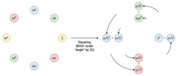
This is the cleverness of Circle STARKs. Given a prime number p, a group of size p can be found, which has a similar two-to-one characteristic.This group is composed of all points that meet certain specific conditions, for example, x^2 mod p is equal to a set of points where a specific value.
These points follow a rule of addition, which you may find familiar with if you have done trigonometry or complex multiplication recently.
(x_1, y_1) + (x_2, y_2) = (x_1x_2 – y_1y_2, x_1y_2 + x_2y_1)
The double form is:
2 * (x, y) = (2x^2 – 1, 2xy)
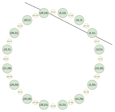
Now, let’s focus on the points on the odd position on this circle:
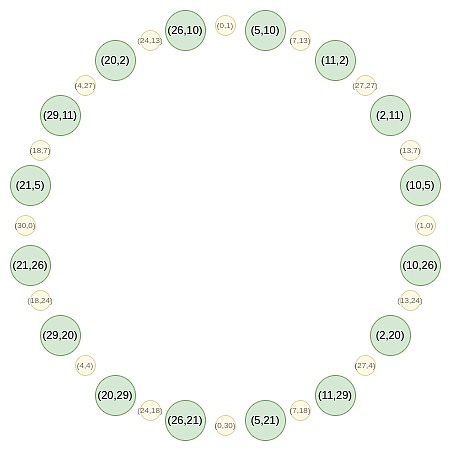
First, we converge all points onto a straight line.The equivalent forms of the B (x²) and C (x²) formulas we use in regular FRI are:
f_0 (x) = \frac {F (x,y) + F (x,-y)}{2}
Then, we can do random linear combinations to obtain a one-dimensional P (x), which is defined on a subset of the x-line:
Starting from the second round, the mapping changed:
f_0 (2x^2-1) = \frac {F (x) + F (-x)}{2}
This mapping actually reduces the size of the above set by half every time, and what happens here is that each x represents two points in a sense: (x, y) and (x, -y).And (x → 2x^2 – 1) is the above point multiplication rule.Therefore, we convert the x coordinates of two opposite points on the circle into the x coordinates of the multiplied point.
For example, if we take the second value of the number from the right of the circle on the second number and apply the mapping 2 → 2 (2^2) – 1 = 7, we get a result of 7.If we go back to the original circle, (2, 11) is the third point from the right, so after multiplying it, we get the sixth point from the right, i.e. (7, 13).
This could have been done in two-dimensional space, but operating in one-dimensional space would make the process more efficient.
Circle FFTs
An algorithm closely related to FRI is FFT, which converts n evaluation values of a polynomial with a degree less than n to n coefficients of the polynomial.The process of FFT is similar to FRI, except that instead of generating random linear combinations of f_0 and f_1 in each step, FFT recursively performs half-sized FFTs on them and takes the output of FFT (f_0) as an even coefficient,Takes the output of FFT (f_1) as an odd coefficient.
Circle group also supports FFT, which is constructed similarly to FRI.However, a key difference is that the objects processed by Circle FFT (and Circle FRI) are not strictly polynomial.Instead, they are what is mathematically called Riemann-Roch space: in this case, the polynomial is modularly circled (x^2 + y^2 – 1 = 0).That is, we treat any multiple of x^2 + y^2 – 1 as zero.Another way to understand it is: we only allow one power of y: Once the y^2 term appears, we replace it with 1 – x^2 .
This also means that the coefficients output by the Circle FFT are not monomial as regular FRI (for example, if the regular FRI output is [6, 2, 8, 3], then we know that this means P (x) = 3x^3+ 8x^2 + 2x + 6).Instead, the coefficients of Circle FFT are the basis for Circle FFT: {1, y, x, xy, 2x^2 – 1, 2x^2y – y, 2x^3 – x, 2x^3y – xy, 8x^4- 8x^2 + 1…}
The good news is that as a developer, you can almost completely ignore this.STARKs never require you to know the coefficients.Instead, you simply store the polynomial as a set of evaluation values on a specific domain.The only place to use FFT is to perform (similar to the Riemann-Roch space) low-degree expansion: Given N values, generate k*N values, all on the same polynomial.In this case, you can use FFT to generate coefficients, append (k-1) n zeros to these coefficients, and then use the inverse FFT to obtain a larger set of evaluation values.
Circle FFT is not the only special FFT type.Elliptic curve FFTs are more powerful because they can work on any finite domain (prime domain, binary domain, etc.).However, ECFFT is more complex and inefficient, so since we can use Circle FFT on p = 2^{31}-1, we chose to use it.
From here we go deeper into some more obscure details, and the details of implementing the Circle STARKs implementation are different from those of regular STARKs.
Quotienting
In the STARK protocol, a common operation is to perform quotient operations on specific points, which can be selected intentionally or randomly.For example, if you want to prove that P (x)=y, you can do it by:
Computing quotient: Given the polynomial P (x) and the constant y, computing quotient Q ={P – y}/{X – x}, where X is the selected point.
Proof polynomial: Proof Q is a polynomial, not a fractional value.In this way, it is proved that P (x)=y is true.
In addition, in the DEEP-FRI protocol, random selection of evaluation points is to reduce the number of Merkle branches, thereby improving the security and efficiency of the FRI protocol.
When dealing with the STARK protocol of the circle group, since there is no linear function that can be passed through a single point, different techniques need to be used to replace the traditional quotient operation method.This usually requires the design of new algorithms using the geometric properties unique to the circle group.
In the circle group, you can construct a tangent function to tangent at a point (P_x, P_y), but this function will have a heavy number of 2 through the point, that is, to make a polynomial theA multiple of a linear function, which must satisfy a stricter condition than being zero only at that point.Therefore, you can’t just prove the evaluation results at one point.So how should we deal with it?
We had to take this challenge, proved by evaluating it at two points, thus adding a virtual point that we don’t need to focus on.
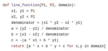
Line function: ax + by + c .If you turn it into an equation and force it to equal 0, then you might recognize it as a line in what is called a standard form in high school mathematics.
If we have a polynomial P equals y_1 at x_1 and y_2 at x_2, we can choose an interpolation function L, which equals y_1 at x_1 and y_2 at x_2.This can be simply expressed as L = \frac {y_2 – y_1}{x_2 – x_1} \cdot (x – x_1) + y_1.
Then we prove that P is equal to y_1 at x_1 and y_2 at x_2, by subtracting L (so that P – L is zero at both points), and by L (i.e., a linear function between x_2 – x_1)Divided by L to prove that the quotient Q is a polynomial.
Vanishing polynomials
In STARK, the polynomial equation you are trying to prove usually looks like C (P (x), P ({next}(x))) = Z (x) ⋅ H (x) , where Z (x) is aPolynomials equal to zero throughout the original evaluation domain.In regular STARK, this function is x^n – 1.In a circular STARK, the corresponding function is:
Z_1 (x,y) = y
Z_2 (x,y) = x
Z_{n+1}(x,y) = (2 * Z_n (x,y)^2) – 1
Note that you can deduce the disappearing polynomial from the collapse function: in a regular STARK you reuse x → x^2 , while in a circular STARK you reuse x → 2x^2 – 1 .However, for the first round, you will do different treatments because the first round is special.
Reverse bit order
In STARKs, the evaluation of polynomials is usually not arranged in “natural” order (e.g., P (ω), P (ω2),…, P (ωn−1), but is based on what I call the inverseReverse bit order:
P (\omega^{\frac {3n}{8}})
If we set n=16 and focus only on which powers of ω we evaluate, the list looks like this:
{0, 8, 4, 12, 2, 10, 6, 14, 1, 9, 5, 13, 3, 11, 7, 15}
This sort has a key property that values grouped together early in the FRI evaluation will be adjacent in the sort.For example, the first step of FRI groups x and -x.In the case of n = 16 , ω^8 = -1, which means P (ω^i) ) and ( P (-ω^i) = P (ω^{i+8}) \).As we can see, these are exactly the right pairs next to each other.The second step of FRI groupes P (ω^i), P (ω^{i+4}), P (ω^{i+8}), and P (ω^{i+12}).These are exactly what we see in four groups, and so on.Doing this makes FRI even more space-saving because it allows you to provide a Merkle proof for values that are folded together (or, if you fold k wheels at once, all 2^k values).
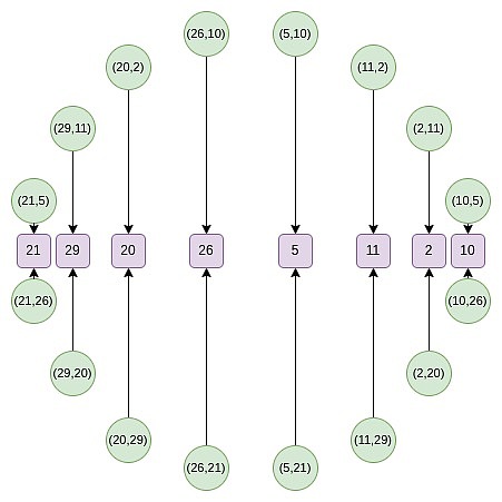
In circle STARKs, the fold structure is slightly different: in the first step we pair (x, y) with (x, -y); in the second step we pair x with -x; in the subsequent stepsIn, pair p with q , select p and q so that Q^i (p) = -Q^i (q), where Q^i is a mapping repeated x → 2x^2-1 i times.If we consider these points from the position on the circle, then in each step, this looks like the first point paired with the last point, the second point paired with the penultimate point, and so on.
In order to adjust the reverse bit order to reflect this folding structure, we need to invert each bit except the last bit.We keep the last bit and use it to decide whether to flip the other bits.
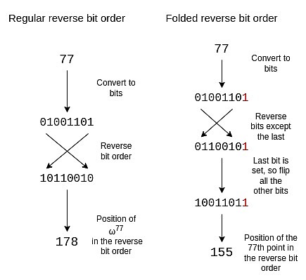
A folded inverse bit order of size 16 is as follows:
{0, 15, 8, 7, 4, 11, 12, 3, 2, 13, 10, 5, 6, 9, 14, 1}
If you observe the circle in the previous section, you will find that the points 0, 15, 8 and 7 (counter-clockwise from the right) are (x, y), (x, -y), (-x, -y) and (-x, y) forms, which are exactly what we need.
efficiency
These protocols are very efficient in Circle STARKs (and generally 31-bit prime STARKs).A calculation proven in Circle STARK usually involves several types of calculations:
1. Native arithmetic: used for business logic, such as counting.
2. Native arithmetic: used in cryptography, such as hash functions like Poseidon.
3. Find parameters: a general and efficient calculation method that implements various calculations by reading values from tables.
The key measure of efficiency is: in computing tracking, do you make the most of the entire space for useful work or leave a lot of free space.In SNARKs in large fields, there is often a lot of free space: Business logic and lookup tables usually involve calculations of small numbers (those numbers are often less than N, N is the total number of calculation steps, and therefore less than 2^{25 in practice}), but you still need to pay the cost of using a bit field of size 2^{256}.Here, the size of the field is 2^{31}, so the wasted space is not much.Low arithmetic complexity hashes designed for SNARKs (such as Poseidon) make full use of every bit of each number in the tracking in any field.
Binius is a better solution than Circle STARKs because it allows you to mix fields of different sizes for more efficient bit packing.Binius also provides the option to perform 32-bit addition without increasing lookup table overhead.However, the price of these advantages (in my opinion) is that they will make the concept more complex, while Circle STARKs (and regular STARKs based on BabyBear) are relatively simple conceptually.
Conclusion: My opinion on Circle STARKs
Circle STARKs Nothing more complicated to developers than STARKs.During the implementation process, the three questions mentioned above are basically the difference from conventional FRI.Although the math behind the polynomials operated by Circle FRI is very complex and it takes some time to understand and appreciate it, this complexity is actually hidden less conspicuously and developers won’t feel it directly.
Understanding Circle FRI and Circle FFTs can also be a way to understand other special FFTs: the most notable are binary domain FFTs, such as the FFTs used by Binius and the previous LibSTARK, and some more complex constructs, such as elliptic curve FFTs, these FFTsUsing a less-to-many mapping can be well combined with the elliptic curve point operation.
Combining Mersenne31, BabyBear, and binary domain technologies like Binius, we do feel like we are approaching the efficiency limits of the base layer of STARKs.At this point, I expect the optimization direction of STARK will have the following key points:
Arithmetic to maximize efficiency of hash functions and signatures: Optimize basic cryptographic primitives such as hash functions and digital signatures into the most efficient form, so that they can achieve optimal performance when used in STARK proofs.This means special optimizations for these primitives to reduce computational effort and increase efficiency.
Perform recursive construction to enable more parallelization: Recursive construction refers to the recursive application of the STARK proof process to different levels, thereby improving parallel processing power.In this way, computing resources can be used more efficiently and the proof process can be accelerated.
Arithmetic virtual machines to improve the developer experience: Arithmetic processing of virtual machines makes it more efficient and simple for developers to create and run computing tasks.This includes optimizing virtual machines for ease of use in STARK proofs, improving developers’ experience when building and testing smart contracts or other computing tasks.